💡This article contains version changes.
Spot the light bulb icon? That means you’ll find helpful details about what’s changed across versions. Read more about version changes here.
The Job Setup page, also referred to as Model Setup, is the interface where users create, view, and manage forecasting jobs and their results.
After uploading a file in Data Management, use Job Setup to generate a forecast based on that file.
The page contains two main sections: an informational section, How Forecasting Works, which provides an overview of the automated forecasting workflow in Board Foresight, and Job Executions, which lists jobs and their results.
To create a forecasting job, click on the Create Job button.
.png)
💡How Forecasting Works
This section explains the four key stages performed behind the scenes to generate forecasts. Each stage includes an information icon that provides additional details about the step.
The How Forecasting Works section is collapsed by default. To expand it, click on the section title.
Time Grid Creation. Missing dates are automatically filled in to create a complete, evenly spaced timeline for each series. All series are expanded to the same global date range, ensuring that the first forecast period starts on the same date across the file.
Feature Engineering. Additional features are generated automatically to help forecasting models identify patterns in the data. These include:
Calendar-based features, such as day of the week and month.
Lag and rolling-window features, including averages and standard deviations of historical values.
Intelligent Routing. Each series is analyzed to determine whether its demand pattern is stable or intermittent. This classification is based on the Median Demand Interval (MDI):
Series with an MDI greater than 0.5 are classified as Intermittent.
Series with an MDI less than or equal to 0.5 are classified as Stable.
Model Assignment. Based on the classification determined during Intelligent Routing, the most appropriate forecasting model is selected for each series:
Stable series are trained and forecasted using Prophet.
Intermittent series are trained and forecasted using LightGBM.
The workflow described in this section applies to jobs created using the Recommended Path. The Recommended Path selects and returns a single forecast generated by the platform's intelligent forecasting engine.
Jobs created using the Univariate Approach follow a separate algorithm-driven workflow. The system prepares the data by completing missing hierarchy combinations and filling missing time periods before running multiple univariate forecasting algorithms in parallel. Instead of returning a single recommended forecast, the Univariate Approach generates forecast outputs from multiple statistical forecasting techniques for the selected hierarchy.
For detailed information on how the forecast engine works, see Forecasting engine overview.
.png)
Create Job
Use this button to create a new job.
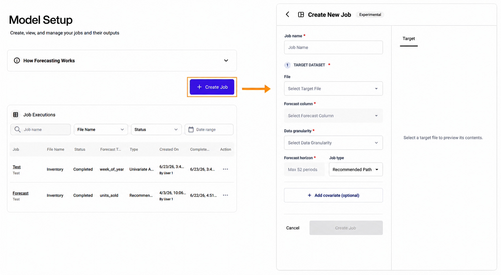
Complete the following fields:
Job name. Enter a name to identify the job.
Target dataset
File. Select a target file to forecast.
Forecast column. Select the column that contains the values to forecast. If multiple numeric columns are available, select the appropriate column from the list.
Data granularity. Define the dimensional level at which the forecast is generated. This setting determines the level of detail of the forecast output.
Forecast horizon. Enter an integer value that represents the number of future periods to forecast.
For daily data, the maximum allowed value is 365 days.
For weekly data, the maximum allowed value is 52 weeks.
For monthly data, the maximum allowed value is 12 months.
The forecast horizon cannot exceed one year based on the selected data frequency.
Job type. Select the forecasting execution path to use for the job. Select one of these two options:
Recommended Path. Choose Recommended Path to use the existing forecasting engine and standard job creation workflow. This path returns a single recommended forecast generated by the platform's intelligent forecasting engine.
For jobs created using the Recommended Path, the platform applies an automated forecasting workflow that prepares the time series, generates features, classifies demand patterns, and selects the most appropriate forecasting model.
💡Univariate Approach. Choose Univariate Approach to use the simplified algorithm driven workflow. This option bypasses the existing forecasting engine and runs multiple statistical forecasting algorithms in parallel rather than a single forecast. Each algorithm produces its own forecast output, allowing results to be compared at algorithm level.The Univariate Approach runs the following forecasting algorithms:
AutoARIMA
AutoETS
ARIMA Airline
Holts Additive
Simple Smoothing
Seasonal Smoothing
Complex Exponential Smoothing
Historic Average
Dynamic Multiplicative Theta
Holts Multiplicative
💡Add covariate (optional)
.png)
💡Covariate dataset. Allows users to add a covariate dataset to the forecast. This option is available only when the Recommended Path job type is selected and is not available for the Univariate Approach.
File. Select a covariate file from the files already uploaded to the system. The list is automatically filtered to show only files classified as Covariate.
Covariate files currently support numeric driver columns only.
Driver column. Select one or more numeric columns from the covariate file to include as external drivers in the forecast. Users can select a single column, multiple columns, or all available numeric columns.
After completing all required fields, review the file previews on the right side of the Create New Job page:
Target. Shows the target file
Covariate. Shows the selected external driver data
Joined. Shows how the target and covariate files are combined using the date and selected hierarchy columns.
.png)
💡Covariate validation requirements
To use a covariate file in a forecast, it must:
Include a date column
Use the same hierarchy columns as the target file
Include at least one numeric column that can be selected as a business driver
Cover the required forecast horizon
Example
if the target file is dimensioned by store and product, the covariate file must use the same dimensions.
If any of these requirements are not met, a validation error appears and the job cannot be created until the issue is resolved.
Once the covariate file passes validation, click Create Job to create and start the forecasting job.
.png)
Job Executions
This section displays all created jobs and their current statuses.
For each job, the following information is available:
Job. Displays the job name.
File Name. Displays the source file used for the job.
Status. Displays the current job status. Available statuses are:
Pending. The job is queued and waiting to start.
Action available: Cancel Job
Training. The model training process is running.
Action available: Cancel Job
Error. The job failed due to an error.
Actions available: Rerun Job or Delete Job.
Forecasting. Model training is complete and forecast generation is running.
Completed. The job finished successfully and results are available.
Actions available: View Results, Rerun Job, or Delete Job.
Canceled. The job was manually stopped during Pending or Training.
Actions available: Rerun Job or Delete Job.
Only completed jobs allow results to be viewed and exported.
Forecast Target. Displays the column selected for forecasting.
💡Type. Displays the forecasting execution path selected when the job was created. Available values are:
Recommended Path
Univariate Approach
Created On. Displays the date and time of creation and the user who created the job.
Completed On. Displays the completion date and time.
Action. Available actions vary according to the job status, as described in each status definition. Available actions can be:
View Results
Rerun Job
Delete Job
.png)
Job Results
When a job status is completed, click on the job name to open the Job Results window.
The Job Results window contains two tabs:
View Job Results
💡Holdout Results
View Job Results
The View Job Results tab displays the generated forecast output and provides options to review, aggregate, filter, and export the forecast data.
.png)
It displays the following information:
Job name and description
Forecast target
Forecast horizon
Records generated
Job creator
Creation and completion dates
External drivers used by the job, when applicable.
External drivers are additional files used by the job. When external drivers are used, they are displayed in the job information area so that the user can confirm which additional files were included in the forecast calculation.
Additional options include:
Row display options. Select the number of rows displayed per page: 25, 100, or 1000.
Calculation method. Select the aggregation method, SUM or AVG, to define how forecast values are aggregated.
The selected calculation method and hierarchy level are applied to all forecast columns, so every algorithm output is recalculated using the same aggregation settings. If aggregation is not supported for the displayed multi-algorithm output, the aggregation controls are hidden.
Displayed items. Select the items to display on the screen.
Frequency. Select the time granularity used to display forecast results: daily, weekly, or monthly.
When the frequency is changed, the platform automatically recalculates and displays the forecast results using the selected time aggregation.
Hierarchy level. Select the hierarchy level at which results are displayed or aggregated. Depending on the data structure, hierarchy columns can include fields such as Item ID, Store ID, location, customer, or other dimensions.
Export CSV. Export forecast results in CSV format.
Forecasting jobs and forecast results are stored in the region assigned to the customer environment.
💡For jobs created using the Univariate Approach, the results include one forecast column for each algorithm that was executed. Column headers correspond to the algorithm identifiers, allowing users to compare algorithm outputs in the same results table. The table displays forecast periods and values at the selected hierarchy level, with each forecasting algorithm producing its own forecast output for side by side comparison and evaluation. See example below:
(1).png)
💡Holdout Results
The Holdout Results tab displays forecast-validation results for jobs created using the Recommended Path only. It helps users evaluate forecast accuracy by comparing forecasted values with actual historical values already available in the target file.
Holdout validation runs automatically when a job is created. Users do not need to configure or run it separately.
.png)
The target file must contain at least three years of historical data for holdout results to be generated.
The holdout period is based on the value selected in the Forecast horizon field during job creation. The platform temporarily excludes an equivalent historical period from the target file, generates a forecast for that period, and compares the forecast with the actual values already available in the file.
Example
if the forecast horizon is 12 months, the platform uses a 12-month historical period as the holdout period.
The Holdout Results tab displays job information, including the job name and description, creator, creation date and time, and job type. It also provides controls for changing the number of rows displayed, calculation method, hierarchy level, and frequency.
The displayed values and holdout metrics are recalculated according to the selected calculation method, hierarchy level, and frequency.
Holdout error
The Holdout error section summarizes forecast performance for the data included in the current selection.
It displays the following metrics:
MAPE (Mean Absolute Percentage Error). Measures the average percentage difference between the forecast and actual values. Lower values indicate greater forecast accuracy. Because MAPE is expressed as a percentage, it is generally easy to interpret. However, it can become unstable when actual values are zero or close to zero.
Forecast Error. Measures the difference between the total actual value and the total forecast value. It helps identify whether the forecast underestimates or overestimates actual demand.
Forecast Error = Total Actual − Total ForecastA positive value indicates under-forecasting because the total actual value is greater than the total forecast value.
A negative value indicates over-forecasting because the total forecast value is greater than the total actual value.
A value of zero indicates that the total actual and total forecast values are equal.
WAPE (Weighted Absolute Percentage Error). Measures the total absolute difference between forecast and actual values relative to the total actual value.
WAPE = Σ|Forecast − Actual| ÷ ΣActualLower values indicate greater forecast accuracy. WAPE is generally more stable than MAPE for files that contain low-volume or intermittent demand because it evaluates the total error relative to the total actual volume.
The WAPE formula remains the same regardless of whether SUM or AVG is selected. However, the calculation uses the actual and forecast values produced by the selected calculation method. Therefore, changing the calculation method may change the resulting WAPE value.
Total actual. Displays the sum or average of the values in the actual column, according to the selected calculation method.
Total forecast. Displays the sum or average of the values in the forecast column, according to the selected calculation method.
.png)